The objectives of this article are to present the basics of Causal Inference, study examples of how a data table can be easily misinterpreted, and discuss how a Data Scientist can incorporate Causal Inference to a Machine Learning pipeline.
The main reference for this article is the book “Causal Inference in Statistics: a Primer” by Pearl, Glymour and Jewell. More bibliography and references are presented at the end of this article.
. . .
Motivation
The development and popularization in recent years of different Machine Learning and Deep Learning algorithms allow us to model very complex relationships and patterns involving a large amount of variables and observations, leading to the implementation of solutions to extremely complex problems.
Most of these complex algorithms yield black box models –that is, models where it is very hard to recover the impact of each input on the output of the model- . If we care only about prediction accuracy, dealing with a black box model should not be a major problem. However, if we detect a scenario where our model under-performs, it is unlikely that we will find out the reason.
When we are not dealing with a black box model, we are usually trying to understand how our different variables interact; in cases where have little prior knowledge about the variables we are modeling, it is hard to rule out a flawed model, and we will most likely be misled by its results, arriving to false conclusions.
Having this in mind, I find that there are two major motivations for any Data Scientist to study Causal Inference:
- Identify different subsets of variables that need to be modeled separately, leading to more control on how and what our models learn.
- Develop tools to avoid misinterpretations of both data tables and results yielded by machine learning algorithms.
Why Causal Inference?
“Correlation does not imply causation”. That is a phrase that every student in any undergraduate probability course heard so many times that, eventually, becomes a mantra that they utter to their students/colleagues/clients later on. As soon as we learn to quantify correlations between variables, we are warned about how easy it is to misinterpret what correlation means. For example, rain and wet street are positively correlated variables, but wetting the street will not make rain happen.
Bayesian and Frequentist Statistics do not provide tools to discern whether rain makes the street wet, or if wetting the floor makes rain happen, or neither. What they can help us with is modeling and quantifying the existing dependence between rain and wet street.
The issue is that, in most problems where data is modeled using Machine Learning algorithms, Data Scientist are expected to provide conclusions such as “rain makes the street wet”. As we know that the data will not yield that kind of results, Data Scientist use to lean on the Field Experts, and on common sense. An Expert can look at the existing dependencies between our variables, and make sense out of them using their vast knowledge of the field. This Field Expert / Data Scientist interaction can drive both an Exploratory Data Analysis and the interpretation of the results yielded by a trained model. And sometimes, the data and results seem to be so clear that common sense could be good enough to make sense out of the data (in the same fashion as we already did with the rain and wet street example).
Sadly, the scenarios where the common sense is not enough, or even when the knowledge of the expert is not vast enough, are far too common. What we would need are statistical tools that guide our understanding on the existing causation between our variables.
A parallelism can be traced with hypothesis tests. Let us put ourselves in Ronald Fisher’s shoes when Muriel Bristol claimed that she could detect whether the milk was poured before or after the tea in her cup, just by tasting it. Fisher decided to prepare 10 cups of tea with milk, where the tea was poured first in only 5 of them. With this information, Muriel Bristol had to taste every cup, and declare whether the tea or the milk was poured first; let us suppose she only made 4 mistakes. Now, how can we conclude from the data if her claim has merits? There are no experts in this peculiar field, and it is hard to assess if 4 mistakes are too many or not. Fisher needed to develop a statistical tool -the Fisher’s Exact Test-, so that the data would yield a statistical conclusion.
Photo by rajat sarki on Unsplash
Causal Inference aims to provide statistical conclusions to causality questions. And this could really help us in some scenarios where the interaction between variables is far too complex, or unexplored.
How does Causal Inference look like?
Causal inference models the interaction of every variable related to our problem -even considering those for which we do not have available data- using a Directed Acyclic Graph (DAG), where every node is a variable, every link indicates a direct dependency, and every link direction indicates the causal flow. So, if X and Y are two variables in our problem, an arrow from X to Y will exist if and only if X is a direct cause of Y.
The variables composing our DAG can be divided in two groups. The exogenous variables are those that are not caused by any other variable; we usually place in this category random variables representing noise, or variables for which we do not have data available. The endogenous variables are the variables that are caused (directly or indirectly) by the exogenous variables; every endogenous variable has to be a variable for which we have data available.
It is important to note that Causal Inference does not care about the shape or amount of dependency between variables, we already have Machine Learning models and algorithms for that task. Causal Inference cares about finding which variables are direct cause of others (is X a cause of Y? It is a yes/no question), and helping us understand the implications of the resulting causal flow.
When inferring the causal DAG from scratch, one possible methodology is to propose different candidate DAGs, and assess their viability by testing conditional or unconditional independence of different pairs of variables; if we obtain results that do not agree with a given DAG, then we discard the latter. As there are so many possible DAGs when the number of variables is large, exploring every possible DAG is computationally expensive; the assistance of Field Experts might help narrowing the search. There is usually not a unique viable DAG, choosing which one we should keep is another problem where a Field Expert could be of great help.
When we already have a DAG, then we could be interested in posing question such as “is X a cause of Y?”. The interventions and do-calculus are tools that will allow us to answer this kind of questions (as long as this causation is identifiable). Long story short, interventions allow us to force the value of a variable in every observation to be constant, and that would answer questions like “if we have a group of sick people, how would the recovery rate change if they are given an experimental drug?”. Obviously, the problem is that we can not give everyone the drug, and at the same time give no one the drug, and compare the results. People are usually split in a control group and an experimental group of the same size, which are studied and compared; using interventions, we can use this data to assess which global scenario yields the largest recovery rate. If the causation is identifiable, we can use do-calculus to compute interventions.
Simpson’s paradox
Let us explore a very simple toy example that can be wildly misleading. The example is extracted from the book “Causal Inference in Statistics: a Primer”, and originally posed by Edward H. Simpson in 1951. The idea is to show how a deep understanding of the causal structure of our variables can help us avoid misinterpretations.
Suppose we want to assess if an experimental drug improves the recovery rate of the patients. As usual, a control group (where people are given no treatment) and an experimental group (where people are given the experimental drug) are assembled, and then we gather the resulting data, which we show in Table 1. As the proportion of men and women are very uneven in both groups, the results are also segmented by sex.
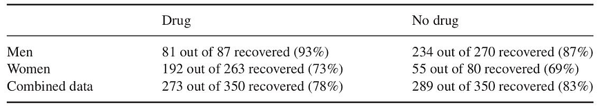
Table 1: Recoveries for the control and experiment group, segmented by sex. The table was extracted from the book “Causal Inference in Statistics: a Primer”.
When we observe the recovery rate by group, we conclude that taking the drug reduces the recovery rate. But when observing by segment, we observe that both women and men have increased recovery rates when taking the drug. So, as a Data Scientist, what should the conclusion be? Should we recommend the drug, even when it decreases the global recovery rate? Or should we not recommend it, even when both women and men benefit from it?
When consulting a doctor who is an expert in this disease, they inform us that we should be aware that estrogen reduces the recovery rate. This can be verified in Table 1. So, when considering the variables drug intake, sex, and recovery rate, we can propose a causal structure following the DAG shown in Figure 1.
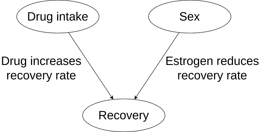
Figure 1: Causal structure for this problem.
We understand now that the experimental group has a lower recovery rate because it has a larger proportion of women, compared to the control group. When analyzing the impact of the drug on each segment, we observe its beneficial properties. The conclusion should be that we recommend the use of the drug.
If you think that this example is too misleading, just imagine how much worse can it get when considering a large amount of variables with complex interactions. Furthermore, we did not discuss how to quantify the contribution of drug intake to recovery rate, we just noted that it is “helping”.
Adding Causal Inference to our Data Modeling
As stated before, Causal Inference is not an alternative to Machine Learning. Quite the contrary, Causal Inference gives us tools and ideas that are complementary to the Machine Learning pipeline.
My ideal pipeline looks something like this:
- Tidying and ordering the data,
- Exploratory Data Analysis,
- Detection of relationships between variables,
- Modeling existing relationships between variables,
- Quantifying existing relationships between variables,
- Conclusions.
As I see it, Causal Inference would greatly help in points 3, 4 and 6. About point 4, I find very interesting the idea of building composite models, where we model interactions between a variable and its direct causes, starting from exogenous variables and building deeper into the causal flow. I think this methodology could yield more robust and interpretable models.
Furthermore, some problems look like “return the list of variables that affect the target variable Y”, which is something that should be attacked mostly using Causal Inference (as we do not care about how they affect Y). Using Machine Learning, these problems could be attacked using interpretable models with variable selection/importance features; but as we see, this might not be the ideal approach.
Bibliography and References
- Causal Inference in Statistics: a Primer. Pearl, Glymour and Jewell, 2016 (book).
- Introduction to Causal Inference from a Machine Learning Perspective. Neal, 2020 (book draft).
- The Do-Calculus Revisited. Pearl, 2012 (keynote lecture).
- Machine Learning for Causal Inference in Biological Networks: Perspectives of This Challenge. Lecca, 2022 (article).
- The Book of Why: the New Science of Cause and Effect. Pearl and Mackenzie, 2018 (book).
- Machine Learning Interpretability. Benbriqa, 2022 (blog).
- Why Data Scientist Should Learn Causal Inference. Ye, 2022 (blog).