The objectives of this article are to present the basics of Causal Inference, study examples of how a data table can be easily misinterpreted, and discuss how a Data Scientist can incorporate Causal Inference to a Machine Learning pipeline.
The main reference for this article is the book “Causal Inference in Statistics: a Primer” by Pearl, Glymour and Jewell. More bibliography and references are presented at the end of this article.
. . .
Motivation
The development and popularization in recent years of different Machine Learning and Deep Learning algorithms allow us to model very complex relationships and patterns involving a large amount of variables and observations, leading to the implementation of solutions to extremely complex problems.
Most of these complex algorithms yield black box models –that is, models where it is very hard to recover the impact of each input on the output of the model- . If we care only about prediction accuracy, dealing with a black box model should not be a major problem. However, if we detect a scenario where our model under-performs, it is unlikely that we will find out the reason.
When we are not dealing with a black box model, we are usually trying to understand how our different variables interact; in cases where have little prior knowledge about the variables we are modeling, it is hard to rule out a flawed model, and we will most likely be misled by its results, arriving to false conclusions.
Having this in mind, I find that there are two major motivations for any Data Scientist to study Causal Inference:
- Identify different subsets of variables that need to be modeled separately, leading to more control on how and what our models learn.
- Develop tools to avoid misinterpretations of both data tables and results yielded by machine learning algorithms.
Why Causal Inference?
“Correlation does not imply causation”. That is a phrase that every student in any undergraduate probability course heard so many times that, eventually, becomes a mantra that they utter to their students/colleagues/clients later on. As soon as we learn to quantify correlations between variables, we are warned about how easy it is to misinterpret what correlation means. For example, rain and wet street are positively correlated variables, but wetting the street will not make rain happen.
Bayesian and Frequentist Statistics do not provide tools to discern whether rain makes the street wet, or if wetting the floor makes rain happen, or neither. What they can help us with is modeling and quantifying the existing dependence between rain and wet street.
The issue is that, in most problems where data is modeled using Machine Learning algorithms, Data Scientist are expected to provide conclusions such as “rain makes the street wet”. As we know that the data will not yield that kind of results, Data Scientist use to lean on the Field Experts, and on common sense. An Expert can look at the existing dependencies between our variables, and make sense out of them using their vast knowledge of the field. This Field Expert / Data Scientist interaction can drive both an Exploratory Data Analysis and the interpretation of the results yielded by a trained model. And sometimes, the data and results seem to be so clear that common sense could be good enough to make sense out of the data (in the same fashion as we already did with the rain and wet street example).
Sadly, the scenarios where the common sense is not enough, or even when the knowledge of the expert is not vast enough, are far too common. What we would need are statistical tools that guide our understanding on the existing causation between our variables.
A parallelism can be traced with hypothesis tests. Let us put ourselves in Ronald Fisher’s shoes when Muriel Bristol claimed that she could detect whether the milk was poured before or after the tea in her cup, just by tasting it. Fisher decided to prepare 10 cups of tea with milk, where the tea was poured first in only 5 of them. With this information, Muriel Bristol had to taste every cup, and declare whether the tea or the milk was poured first; let us suppose she only made 4 mistakes. Now, how can we conclude from the data if her claim has merits? There are no experts in this peculiar field, and it is hard to assess if 4 mistakes are too many or not. Fisher needed to develop a statistical tool -the Fisher’s Exact Test-, so that the data would yield a statistical conclusion.
Photo by rajat sarki on Unsplash
Causal Inference aims to provide statistical conclusions to causality questions. And this could really help us in some scenarios where the interaction between variables is far too complex, or unexplored.
How does Causal Inference look like?
Causal inference models the interaction of every variable related to our problem -even considering those for which we do not have available data- using a Directed Acyclic Graph (DAG), where every node is a variable, every link indicates a direct dependency, and every link direction indicates the causal flow. So, if X and Y are two variables in our problem, an arrow from X to Y will exist if and only if X is a direct cause of Y.
The variables composing our DAG can be divided in two groups. The exogenous variables are those that are not caused by any other variable; we usually place in this category random variables representing noise, or variables for which we do not have data available. The endogenous variables are the variables that are caused (directly or indirectly) by the exogenous variables; every endogenous variable has to be a variable for which we have data available.
It is important to note that Causal Inference does not care about the shape or amount of dependency between variables, we already have Machine Learning models and algorithms for that task. Causal Inference cares about finding which variables are direct cause of others (is X a cause of Y? It is a yes/no question), and helping us understand the implications of the resulting causal flow.
When inferring the causal DAG from scratch, one possible methodology is to propose different candidate DAGs, and assess their viability by testing conditional or unconditional independence of different pairs of variables; if we obtain results that do not agree with a given DAG, then we discard the latter. As there are so many possible DAGs when the number of variables is large, exploring every possible DAG is computationally expensive; the assistance of Field Experts might help narrowing the search. There is usually not a unique viable DAG, choosing which one we should keep is another problem where a Field Expert could be of great help.
When we already have a DAG, then we could be interested in posing question such as “is X a cause of Y?”. The interventions and do-calculus are tools that will allow us to answer this kind of questions (as long as this causation is identifiable). Long story short, interventions allow us to force the value of a variable in every observation to be constant, and that would answer questions like “if we have a group of sick people, how would the recovery rate change if they are given an experimental drug?”. Obviously, the problem is that we can not give everyone the drug, and at the same time give no one the drug, and compare the results. People are usually split in a control group and an experimental group of the same size, which are studied and compared; using interventions, we can use this data to assess which global scenario yields the largest recovery rate. If the causation is identifiable, we can use do-calculus to compute interventions.
Simpson’s paradox
Let us explore a very simple toy example that can be wildly misleading. The example is extracted from the book “Causal Inference in Statistics: a Primer”, and originally posed by Edward H. Simpson in 1951. The idea is to show how a deep understanding of the causal structure of our variables can help us avoid misinterpretations.
Suppose we want to assess if an experimental drug improves the recovery rate of the patients. As usual, a control group (where people are given no treatment) and an experimental group (where people are given the experimental drug) are assembled, and then we gather the resulting data, which we show in Table 1. As the proportion of men and women are very uneven in both groups, the results are also segmented by sex.
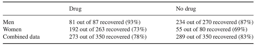
Table 1: Recoveries for the control and experiment group, segmented by sex. The table was extracted from the book “Causal Inference in Statistics: a Primer”.
When we observe the recovery rate by group, we conclude that taking the drug reduces the recovery rate. But when observing by segment, we observe that both women and men have increased recovery rates when taking the drug. So, as a Data Scientist, what should the conclusion be? Should we recommend the drug, even when it decreases the global recovery rate? Or should we not recommend it, even when both women and men benefit from it?
When consulting a doctor who is an expert in this disease, they inform us that we should be aware that estrogen reduces the recovery rate. This can be verified in Table 1. So, when considering the variables drug intake, sex, and recovery rate, we can propose a causal structure following the DAG shown in Figure 1.
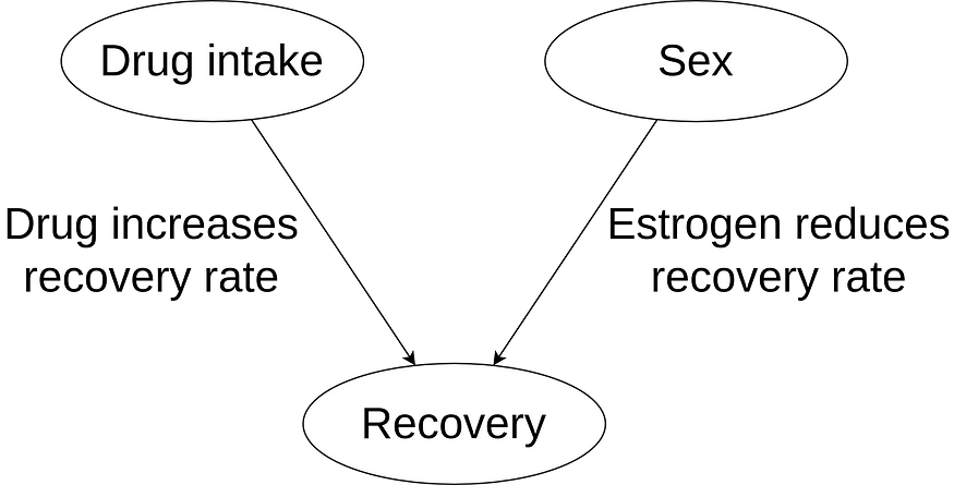
Figure 1: Causal structure for this problem.
We understand now that the experimental group has a lower recovery rate because it has a larger proportion of women, compared to the control group. When analyzing the impact of the drug on each segment, we observe its beneficial properties. The conclusion should be that we recommend the use of the drug.
If you think that this example is too misleading, just imagine how much worse can it get when considering a large amount of variables with complex interactions. Furthermore, we did not discuss how to quantify the contribution of drug intake to recovery rate, we just noted that it is “helping”.
Adding Causal Inference to our Data Modeling
As stated before, Causal Inference is not an alternative to Machine Learning. Quite the contrary, Causal Inference gives us tools and ideas that are complementary to the Machine Learning pipeline.
My ideal pipeline looks something like this:
- Tidying and ordering the data,
- Exploratory Data Analysis,
- Detection of relationships between variables,
- Modeling existing relationships between variables,
- Quantifying existing relationships between variables,
- Conclusions.
As I see it, Causal Inference would greatly help in points 3, 4 and 6. About point 4, I find very interesting the idea of building composite models, where we model interactions between a variable and its direct causes, starting from exogenous variables and building deeper into the causal flow. I think this methodology could yield more robust and interpretable models.
Furthermore, some problems look like “return the list of variables that affect the target variable Y”, which is something that should be attacked mostly using Causal Inference (as we do not care about how they affect Y). Using Machine Learning, these problems could be attacked using interpretable models with variable selection/importance features; but as we see, this might not be the ideal approach.
Bibliography and References
- Causal Inference in Statistics: a Primer. Pearl, Glymour and Jewell, 2016 (book).
- Introduction to Causal Inference from a Machine Learning Perspective. Neal, 2020 (book draft).
- The Do-Calculus Revisited. Pearl, 2012 (keynote lecture).
- Machine Learning for Causal Inference in Biological Networks: Perspectives of This Challenge. Lecca, 2022 (article).
- The Book of Why: the New Science of Cause and Effect. Pearl and Mackenzie, 2018 (book).
- Machine Learning Interpretability. Benbriqa, 2022 (blog).
- Why Data Scientist Should Learn Causal Inference. Ye, 2022 (blog).
This is the third article of the fuzzy logic and machine learning interpretability article series.
In the first article ,we discussed Machine learning interpretability; its definition(s), taxonomy of its methods and its evaluation methodologies.
In the second part of this article series, I introduced basic concepts of fuzzy logic as well as fuzzy inference systems.
This article will build upon the previous ones, and present a new framework that combines concepts from neural networks and fuzzy logic.
. . .
What’s wrong with ANNs?
Artificial neural networks have proved to be efficient at learning patterns from raw data in various contexts. Subsequently, they have been used to solve very complex problems that previously required burdensome and challenging feature engineering (i.e., voice recognition, image classification).
Nonetheless, neural networks are considered black-box, i.e., they do not provide justifications for their decisions (they lack interpretability). Thus, even if a neural network model performs well (e.g., high accuracy) on a task that requires interpretability (e.g., medical diagnosis), it is not likely to be deployed and used as it does not provide the trust that the end-users (e.g., doctors) require.
The problem is that a single metric, such as classification accuracy, is an incomplete description of most real-world tasks.
Neuro-fuzzy modeling
Neuro-fuzzy modeling attempts to consolidate the strengths of both neural networks and fuzzy inference systems.
In the previous article, we saw that fuzzy inference systems, unlike neural networks, can provide a certain degree of interpretability as they rely on a set of fuzzy rules to make decisions (the rule set has to adhere to certain rules to assure the interpretability).
However, the previous article also showed that fuzzy inference systems can be challenging to build. They require domain knowledge, and unlike neural networks, they cannot learn from raw data.
A quick comparison between the two frameworks can be something like this:
- Artificial neural networks: can be trained from raw data, but areblack box
- Fuzzy inference systems: are difficult to train, but can be interpretable
This illustrates the complementarity of fuzzy inference systems and neural networks, and how potentially beneficial their combination can be.
And it is this complementarity that has motivated reasearchers to develop several neuro-fuzzy architectures.
By the end of this article, one of the most popular neuro-fuzzy networks will have been introduced, explained and coded using R.
ANFIS
ANFIS (Adaptive Neuro-Fuzzy Inference System) is an adaptive neural network equivalent to a fuzzy inference system. It is a five-layered architecture, and this section will describe each one of its layers as well as its training mechanisms.
ANFIS architecture as proposed in the orginal article by J-S-R. Jang
Layer 1: Computes memebership grades of the input values
The first layer is composed of adaptive nodes each with a node function:
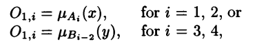
Membership grades
X or y are the input to the node i, Ai and Bi-2 are the linguistic labels (e.g., tall, short) associated with node i, and O1,i is the membership grade of the fuzzy sets Ai and Bi-2. In other words, O1,i is the degree to which the input x (or y) belongs to the fuzzy set associated with the node i.
The membership functions of the fuzzy sets A and B can be for instance the generalized bell function:
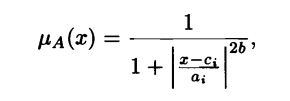
Generalized bell function
Where ( ai, bi, ci) constitute the parameter set. As their values change, the shape of the function changes, thus exhibiting various forms of the membership function. These parameters are referred to as the premise parameters.
Layer 2: Compute the product of the membership grades
The nodes in this layer are labeled ∏. Each one of them outputs the product of its input signals.
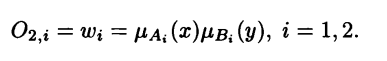
Output of the second layer
The output of the nodes in this layer represents the firing strength of a rule.
Layer 3: Normalization
This layer is called the normalization layer. Each node i in this layer computes the ratio of the i-th rule’s firing to the sum of all rules’ firing strengths:
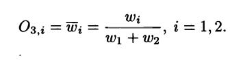
Output of the third layer
The outputs of this layer are referred to as the normalized firing strengths.
Layer 4: Compute the consequent part of the fuzzy rules
Every node i in this layer is an adaptive node with a node function:
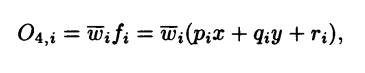
Output of the fourth layer
Where wi is the normalized firing strength of the i-th rule from layer 3 and (pi, qi, ri) constitute the parameter set of this layer. These parameters are referred to as consequent parameters.
Layer 5: Final output
This layer has a single node which computes the overall output of the network as a summation of all the incoming signals.
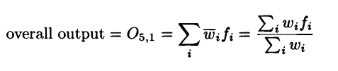
Output of the fifth and final layer
Training mechanisms
We have identified two sets of trainable parameters in the ANFIS architecture:
- Premise parameters: (ai, bi, ci)
- Consequent parameters: (pi, qi, ri)
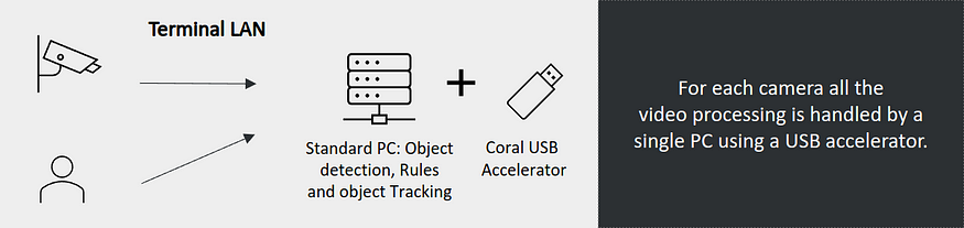
To learn these parameters a hybrid training approach is used. In the forward pass, the nodes output until layer 4 and the consequent parameters are learnt via least-squares method. In the backward pass, the error signals propagate back and premise parameters are learnt using gradient descent.
Table 1: The hybrid learning algorithm used to train ANFIS from ANFIS’ original paper
ANFIS in R
There have been several neuro-fuzzy architectures proposed in the literature. However, the one that was implemented and open-sourced the most is ANFIS.
The Fuzzy Rule-Based Systems (FRBS) R package provides an easy-to-use implementation of ANFIS that can be employed to solve regression and classification problems.
This last section will provide the necessary R code to use ANFIS to solve a binary classification task:
- Install/import the necessary packages
- Import the data from csv to R dataframes
- Set the input parameters required by the frbs.learn() method
- Create and train ANFIS
- Finally, test and evaluate the classifier.
Note that the FRBS implementation of ANFIS is designed to handle regression tasks, however, we can use a threshod (0.5 in the code) to get class labels and thus use it for classification tasks as well!
Conclusion
The apparent complementarity of fuzzy systems and neural networks has led to the development of a new hybrid framework called neuro-fuzzy networks. In this article we saw one of the most popular neuro-fuzzy networks, namely, ANFIS. Its architecture was presented, explained, and its R implementation was provided.
This is the last article of the fuzzy logic and machine learning interpretability article series. I believe that the main takeaways from the three blogs can be:
- Interpretability (in certain contexts) is sometimes of far greater importance than performance.
- There are many ways to assure a certain level of interpretability, one option is to use fuzzy rules to explain the behavior of your machine learning solution.
- Neuro-fuzzy networks are a potential solution to the performance-interpretability tradeoff, it can be worthwhile experimenting with few neuro-fuzzy based architectures.
References
ANFIS: adaptive-network-based fuzzy inference system
This is the second part of the fuzzy logic and machine learning interpretability article series.
In the previous part (here) we discussed Machine learning interpretability; its definition(s), taxonomy of its methods and its evaluation methodologies.
In this second part, we will introduce fuzzy logic and its main components: fuzzy sets, membership functions, linguistic variables, and fuzzy inference systems. These concepts are crucial to understand the use of fuzzy logic in machine learning interpretability.
. . .
Limitations of crisp sets, and the need for fuzzy sets
Classical (or crisp) set theory is one of the most fundamental concepts of mathematics and science. It is an essential tool in various domains, and especially in computer science (e.g., databases, data structures).
Classical set theory relies on the notion of dichotomy: an element x either belongs to a set S or does not. In fact, one of the defining features of a crisp set is that it classifies the elements of a given universe of discourse to members and nonmembers. Crisp sets have clear and unambiguous boundaries.
The belongingness of an element to a set is expressed via a characteristic function.
A characteristic function S(x) of a set S defined on the universe of discourse X has the following form:
(1) S(x)=1 , if x ∈ S and 0 , otherwise
Despite its widespread use, classical set theory still has several drawbacks.
Among them is its incapacity to model imprecise and vague concepts. For instance, let’s say we want to define the set tall people using crisp sets, and we decided to use the following characteristic function:
(2) tallpeople =1 if height>175, 0 otherwise
Meaning that a person is a member of the set of tall people, if their height is greater than 1.75 meters. This definition of the concept of tall leads to unreasonable conclusions. For example, using the characteristic function (2) we deduce that a person whose height is 174.9 cm is not tall, while a person whose height is 175.1 cm is. This sharp transition between inclusion and exclusion sets is one of crisp sets theory’s major flaws, And it is what has led to development and the use of fuzzy sets theory.
Fuzzy logic and fuzzy sets
“As complexity rises, precise statements lose meaning and meaningful statements lose precision”, Lotfi A. Zadeh
Fuzzy logic attempts to resemble the human decision-making process. It deals with vague and imprecise information. Fuzzy logic-based systems have shown great potential in dealing with problems where information is vague and imprecise. They are being used in numerous applications ranging from voice recognition to control.
Fuzzy set theory (introduced in 1965 by Lotfi Zadeh) is an extension of classical set theory. Fuzzy set theory departs from the dichotomy principle and allows for memberships to a set to be a matter of degree. It has gained so much ground because it models better the physical world where most of the knowledge is fuzzy and vague. For example, notions like good, bad, tall, and young are all fuzzy. That is, there is neither a qualitative value, nor a range with clear boundaries that defines them.
Membership functions
Formally, a fuzzy set F is characterized by a membership function mapping the elements of a universe of discourse X to the interval [0, 1].
F :X→0,1
Membership functions map elements of the universe of discourse X to an interval [0,1] where 0 means exclusion, 1 signifies complete membership, and the intermediate membership values show that an element can be a member of two classes at the same time with different degrees. This allows gradual transitions from one class to the other.
The belonging to multiple classes at the same time, and the gradual transition from one class to another, are illustrated in the following example.
Figure 1 shows membership functions of the concept Temperature. In this example, a temperature in celsius can be a member of the following fuzzy sets : Extremely Low, Very low, Low, and Nice temperatures. The X-axis and Y-axis refer respectively to the temperature values in celsius and belongingness percentages. For example, a temperature of 8° is 5% nice and 23% low.
This process of mapping crisp values (such as 8°) to fuzzy values is called Fuzzification. And it is the first step in fuzzy inference systems, more on that later.
Figure 1. Membership functions of the fuzzy sets: extremely low, very low, low, nice temperatures
Linguistic variables
Another fundamental concept of fuzzy logic is linguistic variables. Thanks to linguistic variables (or fuzzy variables), machines can understand the human language, and do inference using our vague and imprecise statements.
A linguistic variable can be defined as a variable whose values are not numbers, but rather, words. Formally, a linguistic variable is defined by the following quintuple:
- X: the name of the variables
- T(X): the set of terms of X
- U: the universe of discourse
- G: the syntactic rule that generates the name of the terms
- µ: the semantic rule that associates each term of X with its meaning
For example, suppose that X is a linguistic variable called Temperature, its set of terms T(X) can be {low, medium, high}, the universe of discourse U can be the interval [-20:55], and the semantic rules are the membership functions of each term.
Fuzzy inference system
Fuzzy sets and linguistic variables allow us to model human knowledge better. However, can machines do inference using the expert knowledge we embedded in them using fuzzy logic?
Fuzzy inference systems do just that.
Given an input and output, a fuzzy inference system formulates a mapping using a set of fuzzy rules (fuzzy rules have the following form If A Then B, where A and B are fuzzy sets).
This mapping allows future decisions to be made and patterns to be discerned in a transparent manner. Fuzzy inference systems are composed of the following components:
- Fuzzifier: converts the crisp input values to fuzzy ones using the membership functions.
- Rule base: stores the fuzzy rules
- Inference engine: performs the fuzzy inference process
- Defuzzifier: transfers the fuzzy inference results into a crisp output.
Figure 2. Main components of a fuzzy inference system.
There are mainly two groups of fuzzy inference systems: Mamdani, and Sugeno (TSK). The difference between the two lies in the consequent part of their fuzzy rules. The consequent part of the Mamdani fuzzy inference system is a fuzzy set. Meanwhile, the consequence of the TSK fuzzy inference system is a mathematical function. This allows the latter to have more predictive power, and the former to have more interpretability.
Example of a fuzzy inference system
To better understand what a fuzzy inference system is, and what it does, let’s discuss the following example of a Mamdani based fuzzy inference system.
We will try to build a fuzzy inference system that takes as input a temperature value, and adjusts the temperature of the Air Conditioner (AC).
- Rule base and membership functions:
To build a fuzzy inference system, a rule base (i.e., a set of fuzzy rules) and membership functions (defining the fuzzy sets) need to be provided. They are usually provided by domain experts.
For the sake of simplicity, let’s use the membership functions in Figure 1. And let’s suppose that our rule base contains the following three rules:
Rule 1: if Temperature is Very Low or Extremely Low Then AC_Command is Very High
Rule 2: if Temperature is Low Then AC_Command is High
Rule 3: if Temperature is Nice Then AC_Command is Normal
- Fuzzification
The first operation that a fuzzy inference system conducts is fuzzification, i.e., it uses the membership functions to convert the crisp input values to fuzzy values.
If our system receives as input the value x=8°, using the membership functions we defined, this value means that the temperature is 5% nice and 23% low. Formally, this can be written as:
U(x=Low)=0.23
U(x=Nice)=0.05
U(x=Very Low)=0
U(x=Extremely Low)=0
- Rules evaluation:
Having fuzzified the input, we can now evaluate the rules in our rule base.
Rule 1: if Temperature is Very Low (=0) or Extremely Low (=0) Then AC_Command is Very High (=0)
Rule 2: if Temperature is Low (=0.23) Then AC_Command is High (=0.23)
Rule 3: if Temperature is Nice (=0.05) Then AC_Command is Normal (=0.05)
- Aggregation and defuzzification:
Aggregation is the process of unifying the outputs of all rules. The values found in the rule evaluation process (0.05 and 0.23) are projected onto the membership functions of AC_Command (Figure 3). The resulting membership functions of all rule consequent are combined.
Finally, defuzzification is carried out. One popular way to conduct defuzzification is to take the output distribution (blue and orange area in Figure 3) and compute its center of mass. This crisp number would be in our example the appropriate degree of the AC.
Figure 3. membership functions of the fuzzy sets Normal, High, Very High AC command
Conclusion
This article covered the basic notions underlying fuzzy logic. We saw how the need for fuzzy sets emerged, and we briefly discussed what fuzzy sets, membership functions, and linguistic variables are. The most important one of all the concepts we saw in this blog (to understand how fuzzy logic is used in machine learning interpretability) is probably fuzzy inference systems.
In the next article (the final), everything we discussed so far will be brought together (ML interpretability and fuzzy logic) to present and discuss what Neuro-Fuzzy architectures are, and how they can be used to tackle the interpretability-performance tradeoff.
References
Department of Computer Engineering, Sharif University of Technology — Fuzzy logic course
Biosignal Processing and Classification Using Computational Learning and Intelligence- Chapter 8 — Fuzzy logic and fuzzy systems
- A. Kalogirou, “Solar Energy Engineering: Processes and Systems: Second Edition,” Solar Energy Engineering: Processes and Systems: Second Edition, pp. 1–819, 2014, doi: 10.1016/C2011–0–07038–2.
- Zhang et al., “Neuro-Fuzzy and Soft Computing — A Computational Approach to Learning and Artificial Intelligence,” International Review of Automatic Control (IREACO), vol. 13, no. 4, pp. 191–199, Jul. 2020, doi: 10.15866/IREACO.V13I4.19179.
Until a few years ago, deep learning was a tool that could hardly be used in real projects and only with a large budget to afford the cost of GPUs in the cloud. However, with the invention of TPU devices and the field of AI at the Edge, this completely changed and allows developers to build things using deep learning in a way that has never been done before.
In this post, we will explore the use of Coral devices, in conjunction with deep learning models to improve physical safety at one of the largest container terminals in Uruguay.
If any of this sounds interesting to you, sit back, and let’s start the journey!!
. . .
The Port of Montevideo is located in the capital city of Montevideo, on the banks of the “Río de la Plata” river. Due to its strategic location between the Atlantic Ocean and the “Uruguay” river, it is considered one of the main routes of cargo mobilization for Uruguay and MERCOSUR . Over the past decades, it has established itself as a multipurpose port handling: containers, bulk, fishing boats, cruises, passenger transport, cars, and general cargo.
MERCOSUR or officially the Southern Common Market is a commercial and political bloc established in 1991 by several South American countries.
Moreover, only two companies concentrate all-cargo operations in this port: the company of Belgian origin Katoen Natie and the Chilean and Canadian capital company Montecon. Both companies have a great commitment to innovation and the adoption of cutting-edge technology. This philosophy was precisely what led one of these companies to want to incorporate AI into their processes and that led them to us.
Motivation
The client needed a software product that would monitor security cameras in real-time, 24 hours a day. The objective was to detect and prevent potential accidents as well as alert them to the designated people. This AI supervisor would save lives by preventing workplace accidents while saving the company money in potential lawsuits.
In other words, this means real-time detection of people and vehicles doing things that can cause an accident. Until now, this was done by humans who, observing the images on the screens, manually detected these situations. But humans are not made to keep their attention on a screen for long periods, they get distracted, make mistakes and fall asleep. That is why AI is the perfect candidate for this job: it can keep its attention 24 hours a day, it never gets bored and it never stops working.
Why is safety so important? A container terminal is in constant motion where trucks and cranes move the goods demanded by the global economy. In this scenario, a fatal accident is just a tiny miscalculation away. ️. Fortunately, these accidents can be avoided by following some safety guidelines.
Time to hands-on
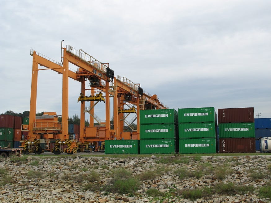
Many things could be monitored and controlled, seeking to reduce the probability of accidents in the terminal. However, the probability can be radically reduced by automatically running the following set of checks against security images:
- Check that every person in image is wearing their PPE (Personal Protective Equipment)
- Check that no vehicle or person is inside an area considered a prohibited area for safety reasons. For instance, the container stowage area or also the marked lanes through which an RTG crane moves. ️️
- Check that no truck, cars or small vehicles move in the wrong direction in the one-way lanes.
- Check that no vehicle exceeds the defined speed limit
Example of RTG Crane (Photo of Kuantan Port on Wikipedia)
To wrap things up, what we need is a system that can access and process the video stream of the security cameras to:
- Detect objects of interest (e.g. vehicles, pedestrians).
- Look for violations to this set of rules.
The diagram below illustrates better the mentioned pipeline.
Solution diagram by IDATHA
Accessing video camera stream, can be done using Python and video processing libraries, easy-peasy. Detecting pedestrians and vehicles and then checking moving directions to finally evaluate an in/out zone rule is more challenging. This can be done using Deep Learning models and Computer Vision techniques.
Accessing video camera stream
IP cameras use a video transmission protocol called RTSP. This protocol has a very convenient particularity: save the bandwidth consumption by transmitting an entire video frame only every certain number of frames. In between, it sends the pixel variations of the previous video frame.
There are some RTSP clients available on the internet which allow you to consume the video stream from an IP camera. We use the client provided by the OpenCV library, implemented in the cv2.VideoCapture class.
Object detection and PPE classification
There are plenty of pre-trained models to detect objects, each with a different trade-off between model accuracy and hardware requirements, as well as execution time. In this project, we had to prioritize performance in detection over hardware requirements because security cameras were far away from the action, making pedestrians and vehicles look too tiny for some models to detect them.
After several performance tests on real images, the winning object detection model was Faster R-CNN, with moderate-high CPU usage, and an average inference time of 500 ms on a cloud-optimized CPU VM (Azure Fsv2 series).
In the case of the PPE classifier there are also several implementations options. In our case we decided to do a Transfer Learning on the Inception model over real images. This approach proved to be very precise and at the same time CPU efficient.
Why not zoom in? Security cameras are part of a closed circuit used by different areas at the company, mainly for surveillance purposes. Consequently, reorienting a camera or zoom was absolutely off the table.
Object Tracking and check safety rules
After calling the Object Detection model, the positions of objects (pedestrians, trucks, etc.) can be compared with the coordinates of the prohibited areas (for example, the container stowage area) and checked if any of them violate any rule. However, a piece of the puzzle is still missing: a method to track the same recognized object over time (consecutive frames in stream).
With a method like this, a pedestrian inside a prohibited area can be detected when he enters, then tracked until he leaves, triggering a one-time alert. There are several models and methods to address this problem, also known as Object Tracking. We used Centroid Tracker algorithm as it showed the best test results.
Framework selection (spoiler alert: it is TensorFlow)
As with pre-trained models, there are several frameworks for working with deep learning; two of the best known and most mature are PyTorch and TensorFlow. In particular, we chose TensorFlow for the following reasons:
- Maturity of the suite.
- Tensorflow Optimization Toolkit, which helps reducing memory and CPU usage.
- Native support for Coral TPU devices.
However, this doesn’t mean that PyTorch would have been a bad choice. We would have changed the hardware option, since PyTorch doesn’t support Coral, but we could have tested it on the NVIDIA Jetson Nano device.
Coral vs. Cloud vs. Servers: the scale factor story
For the sake of an early production release, the first deployment used GPUs servers in the cloud. More in detail, an Azure NC6 VM was used (read more about NC series here). According to the official documentation, this VM has 1 virtual GPU = half NVIDIA TESLA K80 card.
Initially, the hardware was sufficient to process the images from the first 2 cameras. However, time revealed two limitations of this deployment:
- Processing the images in the cloud, saturated the terminal network bandwidth with the video uploading.
- More important, the solution scale factor was 1 NC6 VM (1 virtual GPU) for every 4 new cameras.
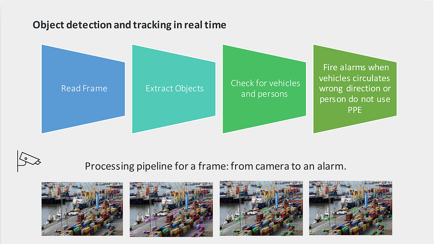
This scenario is where Coral (Google’s TPU devices) kicked the board.
With an initial investment of around USD 100 and no monthly costs, these devices can be installed in the terminal without consuming network upload bandwidth. Also, by optimizing detection models for TPU, using TensorFlow Lite, inference times are reduced around 10x. In this way, the scaling factor changes to a new Coral device every 10 new cameras approximately.
Deployment using Coral by IDATHA
Quick recap!
Let’s quickly summarize all the things we have mentioned about the problem and the solution :
- Safety is enhanced by automatically analyzing frames against object rules.
- Video stream images are accessed through RTSPusing OpenCV library.
- Pedestrians, trucks among others are detected using Faster R-CNN
- Mandatory use of PPE is checked using an image classifier model based on Inception.
- Centroid Trackeralgorithm is used to track objects throw time in video.
- Coraltogether with TensorFlow Lite allows running the model with high performance in situ.
Conclusions
Based on the results obtained by the models, performing the observation and surveillance tasks, we can affirm that the solution is a huge success:
- The models used in this project can perform the same tasks previously performed by security guards, with a higher level of reliability, all day long, maintaining the same performance and no rests.
- More central, surveillance is tedious, monotonous, and could have a detrimental effect on health. Relieving the security guards in these specific tasks, we free them to focus on more challenging labors that require higher skills and cannot be carried out by machines.
- Advances in the field of AI at the Edge, and in particular Coral devices, allow us to develop a low-cost solution. According to our calculations for this project, cloud-based solutions are at least 7x more expensive than Coral.
Undoubtedly there are working lines that weren’t explored that can potentially improve the solution in both performance and operational costs
— but you know who I think could handle a problem like that: future Ted and future Marshall —
Gone are the days when artificial intelligence seemed out of reach and almost exclusive for films. Today, companies that want to scale and boost their efficiency should know how to harness the power of AI. Here at IDATHA, we want to help you tap in and venture into the complicated world of artificial intelligence. Based in Montevideo, Uruguay, our team is filled with passionate professionals dedicated to machine learning, data engineering, computer vision, natural language processing, and so much more.
Because of our proven track record in the space, we’ve made a name for ourselves in the cutthroat industry. Just recently, we caught wind that we’ve been recognized as a leader on Clutch’s 2022 Awards cycle! IDATHA was officially hailed as one of the finest artificial intelligence partners from Uruguay!
“We are very proud to receive the Clutch leader award. This is proof that we are continuously providing the highest quality to our clients.”
Chief Executive Officer of IDATHA
Thank you so much to everyone of our clients who helped us get to where we are today. It’s been a great pleasure working with you and serving as your trusted partner. Your kind words serve as catalysts for our success and recognition.
IDATHA is proud to be a Clutch leader and a five-star team! Turn your data into cutting-edge competitive advantage. Send us a message today and tell us more about what you need. We look forward to working with you!